
The four terms in the title are often abused, sometimes confused, and generally not completely understood. Therefore, the following short descriptive generic descriptions are offered as a first step to clarify this situation.
By: Robert D. Larrabee
Microelectronics Dimensional Metrology Group
National Institute of Standards and Technology
Gaithersburg, Maryland 2O899
I. Precision (i.e., repeatability)
Instrumental precision is often defined as the spread of values obtained with repeated measurements on a given specimen [1-2]. It is generally assumed that the number of repeated measurements is large, that the spread of values obtained is due to random causes, and that randomness results in a Gaussian or “normal’ distribution of measurement data about a mean value. If these assumptions are true, a multiple of the root-mean-square of the measured deviations about this mean can be taken as a measure of the instrumental precision appropriate for that given specimen and for the conditions under which it was measured. Since there are no generally accepted conditions for those measurements, there are a number of different types of precision that can be defined (e.g., short-term, long-term, instrumental, precision attained using different specimens or with different operators, etc.). Therefore, when quoting a precision value, it is important to specify the conditions under which that quoted value was measured and the method used for its calculation. In this way, the user can determine if the quoted precision value is appropriate for the intended application. Basically, precision is a measure of repeatability of a measurement with some things held constant and, perhaps, other things inadvertently or intentionally allowed to vary.
II. Accuracy (i.e., correctness of mean value)
Accuracy is defined as the correctness of a measurement or of the mean of repeated measurements [1-2]. Unfortunately, there are usually many potential sources of nonrandom systematic errors that affect the mean of repeated measurements. Since these systematic errors remain constant from measurement to measurement, they cannot be reduced by averaging the results of repeated measurements. Therefore, systematic errors can lead to significantly incorrect measurement results regardless of the precision of the instrument used. Therefore, good precision is a necessary condition for good accuracy, but not a sufficient condition, The concept of correctness assumes that there is some agreed upon standard which can be used to determine the correctness of a measurement. The desired accuracy may be achieved only if the instrument being calibrated is sufficiently precise, if the standard of comparison is calibrated with sufficient accuracy, and if the specimens of interest exactly match the standard of comparison in all-important ways. One method of using standards is to prepare a calibration curve using a set of standards with a range that includes the desired range of that parameter of interest. Note, however, that it is not good practice to extrapolate this curve outside the range of the standards used in the calibration. Assuming that the standard itself has been prepared with sufficient accuracy, calibration is essentially a measurement of the systematic error of the instrument being calibrated. This calibration can never be more accurate than the standard used and, in general, the calibration will be inferior to the standard because of the inevitable imprecision of the measurements made during the calibration procedure. Another way of looking at this is to consider the instrument in question to be a comparator that compares the unknown to a standard. Therefore, it requires a high quality comparison standard and a high precision instrument (comparator) to give a high quality result.
III. Uncertainty (i.e., how far off is measurement result from true value)
Figure 1 (from [3]) shows diagrams of the probability distribution of the measurements used to calibrate a standard (right-hand distribution with mean Xs) and of the measurements used by a user of the standard in calibrating an instrument (left-hand distribution with mean Xm). The “true” value Xt is also shown in Fig. 1 although, in practice, this value is not known. The uncertainty in both of these two measurements is some appropriate sum of the random and systematic errors (i.e., an appropriate combination of imprecision and inaccuracy). The imprecision is often measured by three times the standard deviation (sigma) of the probability distribution (as estimated by S, the RMS fluctuation of repeated measurements about their mean), and the uncertainty measured by the 3-sigma imprecision added algebraically to the systematic error (i.e., U=E+3S in Fig. 1). Notice that there are random and systematic errors associated with the calibration of the standard and, as a result, a measurement system cannot be calibrated to an uncertainty less than the uncertainty of the standard to which it is compared. Indeed, in Fig. 1, calibration has reduced the systematic error of the user’s instrument from U to U’. Notice, however, that the variance of this calibration is the sum of the variances of calibration of the standard (S’ squared) and the calibration of the instrument (S squared). Because of this compounding of imprecision, calibration measurements of standards and instruments should be done as precisely and carefully as possible (i.e., with small S and S’). Indeed, this compounding of imprecision occurs once again when the calibrated instrument is then used to measure an unknown specimen. Therefore, the uncertainty associated with the actual use of a calibrated instrument is an elusive concept depending on the precision and accuracy of calibration of the standard of comparison, the precision of the calibration of the user’s instrument, and the precision of the user’s instrument in making the measurement of the unknown specimen. In any event, the uncertainty of measurement is not equal to the precision determined by the spread of the measurement results on the unknown specimen’
IV. Traceability (i.e., shifting the problem to someone else)
Traceability is the ability to demonstrate conclusively that a particular instrument or secondary calibration standard is accurate relative to some generally accepted reference standard and, therefore, that subsequent measurements can be ‘traced back” to that standard. For dimensional measurements, the ultimate standard is the International Meter as defined currently by a standardized velocity for light in vacuum. The National Institute of Standards and Technology (NIST, formally the National Bureau of Standards or NBS) has the charter to provide means for establishing traceability to this international standard. Traceability, in this case, can be achieved if a particular instrument or artifact has been calibrated by NIST at accepted intervals or has been calibrated against another standard in a chain of calibrations ultimately leading to a calibration performed by NIST [5]. The emphasis on traceability is important because it enables measurement consistency from laboratory to laboratory in a logical and consistent manner. In-house control specimens can act as interim precision standards but, if and only if, they closely match the specimens to be measured and are known to be stable with time. Unless properly calibrated, these in-house standards do not meet the requirements for accuracy or traceability, but are useful to monitor and to control precision. The necessity to match the properties of the standard to the specimen of interest presents one of the more serious problems to NIST in the development of accurate sub-micrometer standards. Since there are so many different types of specimens of interest with many different thicknesses, edge geometries and physical properties, it would be impossible for NIST to produce a sufficient variety of standards so that everyone will be able to find one that matches any given specimen of interest. Another serious problem in the generation of sub-micrometer dimensional standards is that the metrology necessary for their calibration simply may not exist. This situation has arisen because the development of techniques for sub-micrometer patterning has evolved faster than the development of the corresponding metrological techniques for the accurate measurement of those patterns.
V. What is worse than no metrology? (i.e., no way to measure it accurately)
The present state of the art in sub-micrometer dimensional metrology is that relatively precise instrumentation is commercially available, but the standards required to calibrate those instruments for accuracy may not be available. Therefore, dimensional measurement results should be interpreted with this in mind. For example, a measured deviation of the width of a photo resist line from the desired value may, or may not, be due to an actual deviation in the width of the line. This should not be a surprising result with an instrument that may be inaccurate (i.e., not measure the ‘true” width of the line). For example, this situation could arise when there are changes in other factors that influence the measured “width” value [3-4] (e.g., thickness of the resist, change in the dimensions or optical constants of the substrate structures, change in edge geometry of the resist line, etc.). In other words, without accuracy, it may be improper to interpret the measurement result as actually measuring the parameter of interest (width in this case). Is metrology useful if it may be inaccurate and thus easily misinterpreted in this way? Indeed, is metrology useful if used to adjust the process being monitored by the inaccurate instrument (e.g., adjusting the patterning process to bring the “line width” back to the desired value when it really was the index of refraction of the resist that really changed)? Misinterpreted metrology is bad metrology, and that is one thing that is worse then no metrology! Therefore, it pays to be careful in interpreting the results of uncalibrated (and thus probably inaccurate) instruments!
VI. References
1. ASTM Manual on Presentation of Data and Control Chart Analysis, STP15D, American Society for Testing and Materials, 1916 Race Street, Philadelphia, PA 19103.
2. Many ASTM standards relate to the definition or determination of precision and/or accuracy. These can be found by looking up these two terms (i.e., “precision’ and ‘accuracy”) in the ASTM Annual Book of Standards, Volume 00.01, Subject index; Alphanumeric List, Issued yearly by ASTM.
3. Nyyssonen, D. and R. D. Larrabee, “Sub-micrometer Line width Metrology in the Optical Microscope,’ Jour. of Research of the National Bureau of Stds. (now called the National Institute of Stds. and Technology), Vol. 92, 187-203, May-June, 1987.
4. Postek, M. T., and D. C. Joy, “Sub-micrometer Microelectronics Dimensional Metrology: Scanning Electron Microscopy,” Jour, of Research of the National Bureau of Standards (now called the National Institute of Stds. and Technology), Vol. 92, 205-227, May-June, 1987.
5. Belanger, Brian C., ‘Traceability: An Evolving Concept,” Standardization News, Vol. 8, No. 1 (1980), American Society for Testing and Materials, Philadelphia, PA.
Definition of uncertainty, U, and standard deviation, S. In this figure: Xt is the “true’ value of desired value of the measurement; Xs is the value assigned to the standard with its precision given by 3S’ and total uncertainty, U’; Xm is the result of measurement on another system with precision 3S. If the measurement offset, O, is eliminated by correction to the value of the standard, Xs, the uncertainty, U, associated with Xm is still at least U’.SS. Note that Xt is frequently ill-defined and that when the characteristics of the standard used to determine the offset, O, do not match those of the part to be measured, the uncertainty in Xm may actually be larger than indicated.
SUBMICROMETER OPTICAL METROLOGY*
Robert D. Larrabee
National Bureau of Standards, Gaithersburg, Maryland 20899
The National Bureau of Standards (NBS) has had a continuing program for over 10 years [1-5] to develop optical feature-size standards for the integrated-circuit industry. As the dimensions of interest to this industry have evolved into the sub-micrometer region, feature-size measurements have become more difficult because the dimensions of interest have become comparable to (or smaller than) the wavelength of light used for their measurement. In this domain of feature sizes, diffraction produces large effects in the optical image and makes that image difficult to interpret. The effects of diffraction mask the location of the feature edges that define the dimensions of interest. The fundamental nature of the problem is well illustrated by noting that the Airy disk diameter is 0.45 micrometers for f/1 optics at the near ultraviolet wavelength of 0.366 micrometers, and that the Airy disk diameter is even greater for larger f/# optics in the visible. This image-interpretation (or edge-location) problem is not unique to the dimensional measurements in the semiconductor Industry, but is generic to all sub-micrometer dimensional measurements and, unless it can be proven otherwise, must be considered to play a dominant role in all modes of operation of optical microscopes (e.g., conventional, confocal, focused laser beam, Fourier’ transform, etc.). In this presentation, the basic obstacles that must be overcome to achieve precision and accuracy for sub-micrometer feature-size measurements will be surveyed and the present (and projected future) standards for micrometer and sub-micrometer optical dimensional metrology will be discussed.
References
1. Nyyssonen, Diana and Larrabee, R. D., ~ Linewidth Metrology In the Optical Microscope,” Jour. Research, Nat. Bur. Stds., 92(1987)187.
2. Larrabee, R. D., “Sub-micrometer Optical Line width Metrology,’ Proc. of the Society of Photo-Optical Instrumentation Engineers (SPIE), Volume 775, “Integrated Circuit Metrology, Inspection, and Process Control” Edited by Kevin M. Monahan, March 4-6, 1987, Santa Clara, California, pp. 46-50.
3. Nyyssosnen, D., ‘Metrology in Microlithography,’ Chapter 7 in VLSI Electronics Microstructure Science, Microlithography for VLSI, Vol 16, N.G. Einspruch, Editor, pp. 265-317 (Academic Press, New York, NY, 1987).
4. Bullis, W. M. and Nyyssonen, D., “Optical Linewidth Measurements on Photomasks and Wafers,’ Chapter 7 in VLSI Electronics: Microstructure Science Semiconductor Microlithography, Vol. 3, N. U. Einspurch, Editor, pp. 119-126 (Academic Press, New York, NY, 1982).
5. Nyyssonen, D., “Spatial Coherence: The Key to Accurate Optical Micrometrology, Proc. Soc. Photo-Optical Instrum. Engrs., Applications of Optical Coherence 194(1979)34.
* Contribution of the National Bureau of Standards, not subject to copyright.
Additional References
I. Factors that affect the image in optical sub-micrometer dimensional metrology
1. Nyyssonen, D., “Linewidth Measurement with an optical microscope:
Effect of Operating Conditions on the Image Profile,” Appl. Optics
16(1977)2223.
2. Kirk, C., “A study of Instrumental Errors in Linewidth and Registration Measurements Made with an Optical Microscope,’ Proc. Soc. Photo-Optical Instrum. Engs., Vol. 775, ‘Integrated Circuit Metrology, Inspection and Process Control, Edited by Kevin M. Monahan, March 4-6 1987, Santa Clara, California, pp. 51-59.
3. Kirk, C., “Aberration Effects in an Optical Measuring Microscope,” Appl. Optics 26(1987)3417.
4. “Standard Practice for Preparing an Optical Microscope for Dimensional Measurements,” F728-81, Annual Book of ASTM Standards, American Society for Testing and Materials, Philadelphia, PA, Issued yearly.
II. Theoretical modeling of the image profiles in optical microscopy
1. Nyyssonen, D., ‘Theory of Optical Edge Detection and Imaging of Thick Layers,” Jour. Opt. Soc. Am. 72(1982)1425.
2. Kirk C. P. and Nyyssonen, D., “Modeling the Optical Microscope Images of Thick Layers for the Purpose of Linewidth Measurement,’ Proc. Soc. Photo-Optical Instrum. Engs., Vol. 538, “Optical Microlithography IV,” pp. 179-187 (1985).
3. Nyyssonen, D., “A Practical Method for Edge Detection and Focusing for Linewidth Measurements on Wafers,” Proc. Soc. Photo-Optical Instrum. Engs., Vol. 5389 “Optical Microlithography IV,” pp. 172-178 (1985).
4. Nyyssonen, D., “Computer Software for the Computation of the Scattered Field and the Optical Microscope Image of Line Objects Patterned in Thick Layers,’ NBSIR 87-3618, National Bureau of Standards, Gaithersburg, MD (1987).
III. Line width Standards from NBS
1. Swyt, Dennis A., “An NBS Physical Standard for the Calibration of Photo mask Line width Measuring Systems,’ Proc. Soc. Photo-Optical
Instrum. Engs., Vol. 129, “Effective Utilization of Optics in Quality Assurance,” pp. 98-105 (1978).
2. Croarkin, C. and Varner, R. N., “Measurement Assurance for Dimensional Measurements on Integrated-Circuit Photo masks,” NBS Tech. Note No. 1164, National Bureau of Standards, Gaithersburg, MD (1982).
3. Jerke, 4. M. et al., “Semiconductor Measurement Technology:
Interlaboratory Study on Linewidth Measurements for Antireflective Chromium Photo masks,” NBS Special Publication 400-74, National Bureau of Standards, Gaithersburg, MD (1982).
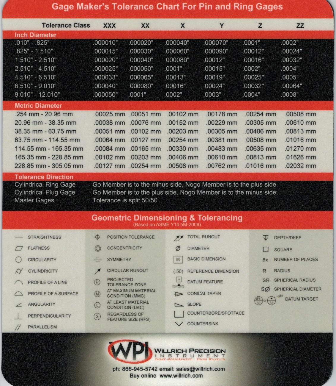
FILL IN BELOW TO RECEIVE YOUR FREE MOUSEPAD OF GAGEMAKERS TOLERANCE AND GD&T SYMBOLS